Groundwater damage Accounting
TR-EX Kalk
Hello dear interested parties,
with the following explanations, I will explain to you the services you will receive when you have me calculate your groundwater damage. Based on the relative location of the measuring points to each other, the measurement values, and the hydrogeological boundary conditions, I will calculate the average pollutant concentration in the source and plume, the pollutant load that flows out of the contaminated groundwater aquifer, and the amount of pollutant mass present in the pore water at the time of measurement.
Concept cloud:
Groundwater Monitoring Wells (GWM), Pollutants, Threshold Limit, Groundwater Flow Direction, Groundwater Thickness, Fracture Percentage, Separating Layer Void, Pore Volume, Porosity, Darcy, Permeability Coefficients, Filter Velocity, Hydraulic Gradient, Groundwater Slope, Balance Level, Minimum Flow Rate (MNQ).
To calculate the pollutant balance, I require the following information from you:
- Coordinates or site plan of the groundwater monitoring wells
- Measurement values of the pollutant being assessed in the groundwater monitoring wells
- Groundwater flow direction
- Groundwater thickness
- Fracture percentage/separating layer void/pore volume/porosity
- Permeability coefficient/filter velocity
- Hydraulic gradient/groundwater slope
- Distance from the pollutant source to the relevant balance level and, if applicable, to a nearby surface water
- Possible average minimum flow rate (MNQ) of the surface water
With this data, I will calculate the following assessment-relevant criteria for you:
- Extent of the groundwater damage
- Volume of the groundwater damage
- Average pollutant concentration and exceedance factor of the threshold limit value
- Average concentration flowing out of the respective balance level
- Daily pollutant load flowing out in the balance level
- Pollutant load flowing into a surface water
- Trends in the individual groundwater monitoring wells as well as in the entire balancing area
- Possible break-even or falling below the threshold limit value.
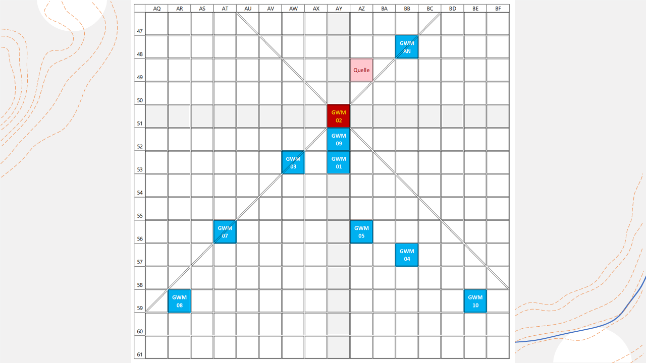
Monitoring point grid/ Monitoring point matrix
Using the coordinates of the groundwater monitoring points provided by you or a georeferenced map, and the measured pollutant concentrations in each groundwater monitoring point, I calculate a grid using a calculation algorithm I have developed, which halves the pollutant concentrations in the respective groundwater flow direction.
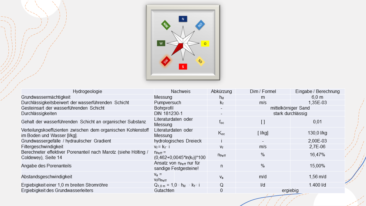
Hydrogeologie
To apply Darcy's law, I only need the values for permeability (kf), groundwater thickness (hGW), and hydraulic gradient (i) from you.
Calculation grid
These data are used to calculate the following assessment-relevant criteria for groundwater damage:
- Area extent of the groundwater damage
- Volume of the groundwater damage
- Average contaminant concentration and the exceedance factor of the GFS value
- Average concentration flowing out of the respective balance level
- Daily outflow of pollutants at the balance level
- Inflowing pollutant load into a surface water body
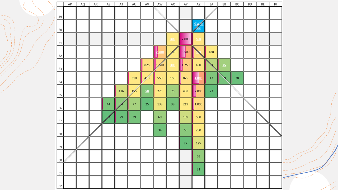
The plume is divided into square grid cells in the form of a computation grid. With each increasing grid distance from the source, the plume is widened by one new cell on both sides. This results in a lateral spreading of the plume at 45° to the main groundwater flow direction. If the spreading calculation is stopped due to the test value falling below the limit, no further widening takes place. The transfer of pollutant concentrations from the considered grid row to the more distant grid rows is done with a calculation algorithm that has been tested with examples. This involves calculating the extrapolation value for the new grid cell in each cell of the new more distant grid cell, based on the distance and the concentrations above it from the three symmetrically upper cells of the previous grid row. However, if a pollutant concentration is already known in a cell because a groundwater measuring point with an actual measured value is located there in the grid, this actual measured value takes precedence over the purely theoretically calculated estimated value. It is important to note that estimated values are uncertain and do not reflect the actual values. Therefore, they should always be treated with caution and not considered as definitive values.
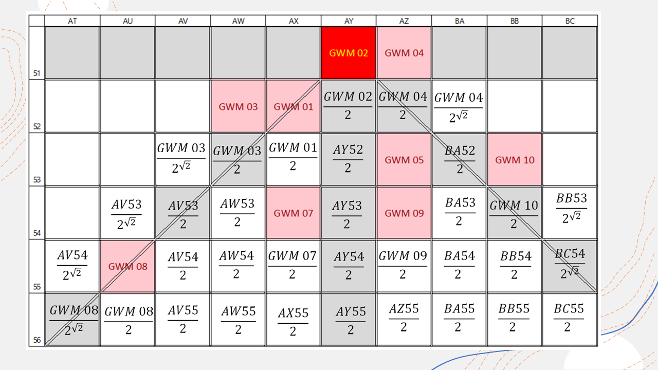
The extrapolation value for grid cells within the same flow tube is calculated using the following formula:
c(below) = c(above) / e^s*lambda = c(above) / 2
The extrapolation value for grid cells outside the same flow tube is calculated using the following formula:
c(below) = c(above) / e^s*lambda = c(above) / 2^√2
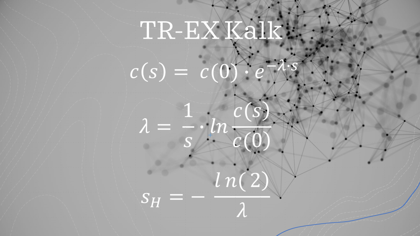
Pollutant degradation equation
Pollutant degradation gradient
Halfing distance
In the calculations, a functional equation is used to compute the concentration profile from one grid cell to the next or from one subregion to another. The concentration loss is proportional to the source concentration c(0) of the pollutant, depending on the geometric distance s of the respective calculation cell. The pollutant degradation equation takes into account all relevant factors influencing the degradation process, such as sorption (attachment of the pollutant to soil particles), desorption (release of the pollutant from soil particles), diffusion (spread of the pollutant in groundwater), dilution, and biological degradation. These factors are considered depending on the physical and chemical properties of the respective pollutant and the environmental conditions in the model space.
The pollutant degradation equation is used to determine the corresponding proportionality factors or concentration gradient reductions for all measurement point combinations. By substituting the value ½ c(0) for c(s) in the pollutant degradation equation and solving the equation for s, one obtains the so-called halfing distance sH, which is the distance at which the pollutant concentration halves. The grid cell is also used to determine the width of a stream tube.
LAWA / LABO Diagram
"According to the enforcement experience of some German federal states, a groundwater contamination is considered to be just small if the contaminated volume does not exceed the order of 100,000 m³ (reference volume) and the contamination with a pollutant on average is not greater than 10 times the concentration of the GFS [B 16]."
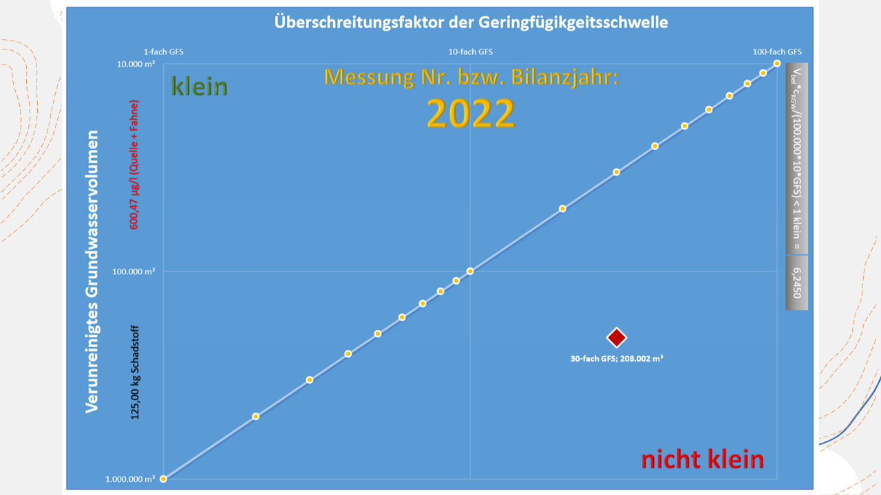
The groundwater damage is not small, as the red diamond is located below the dividing line "small" and "not small".
The average pollutant concentration is the average content of the pollutant in the source and plume of the groundwater contamination. It is used to quantify the average contamination of groundwater by pollutants. The calculation according to the above-mentioned calculation algorithm is terminated if the insignificance threshold is not exceeded. The sum of concentrations in the grid cells with values above the insignificance threshold, divided by the number of grid cells, results in the average pollutant concentration of the groundwater damage (cKGW).
The determined number of cells with GFS exceedance, multiplied by the water-filled volume of a grid cell (square of the half-life distance multiplied by the height of the aquifer and porosity), yields the volume of the source and plume with exceedance of the insignificance threshold. Based on this volume, it can now be estimated whether the groundwater damage is locally limited within the meaning of § 4 (7) BBodSchV [R 02] or § 15 (8) BBodSchV [R 04].
Representation of a damage case with two sources of pollutants in a 2D diagram
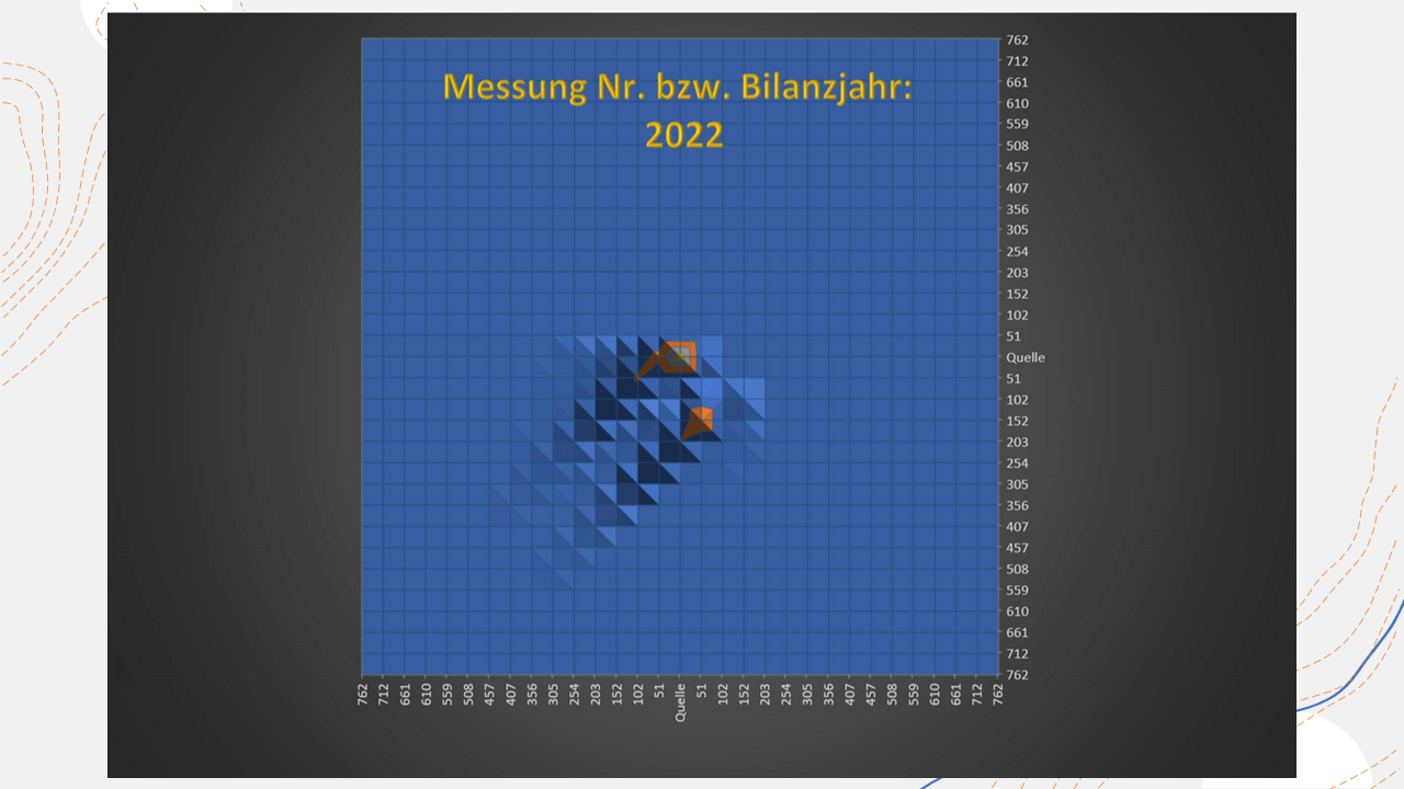
In the above 2D diagram, a groundwater contamination is shown that has spread from northeast to southwest, originating from two sources of pollutants.
Representation of a damage case with two sources of pollutants in a 3D diagram
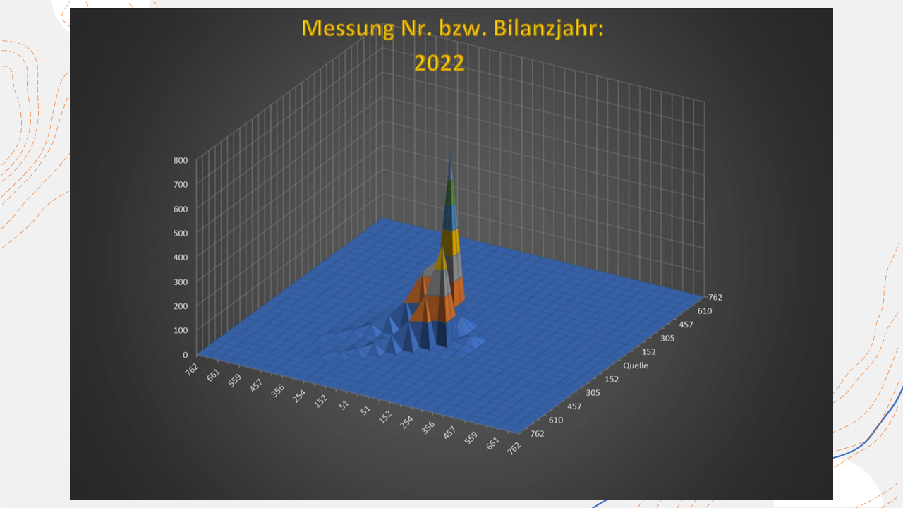
In the above 3D diagram, a groundwater contamination is shown that has spread from northeast to southwest, originating from two sources of pollutants.
The different representations of the contaminant plumes in the diagrams serve to control and deepen the understanding of the process.
Accumulated loads perpendicular to the direction of groundwater flow
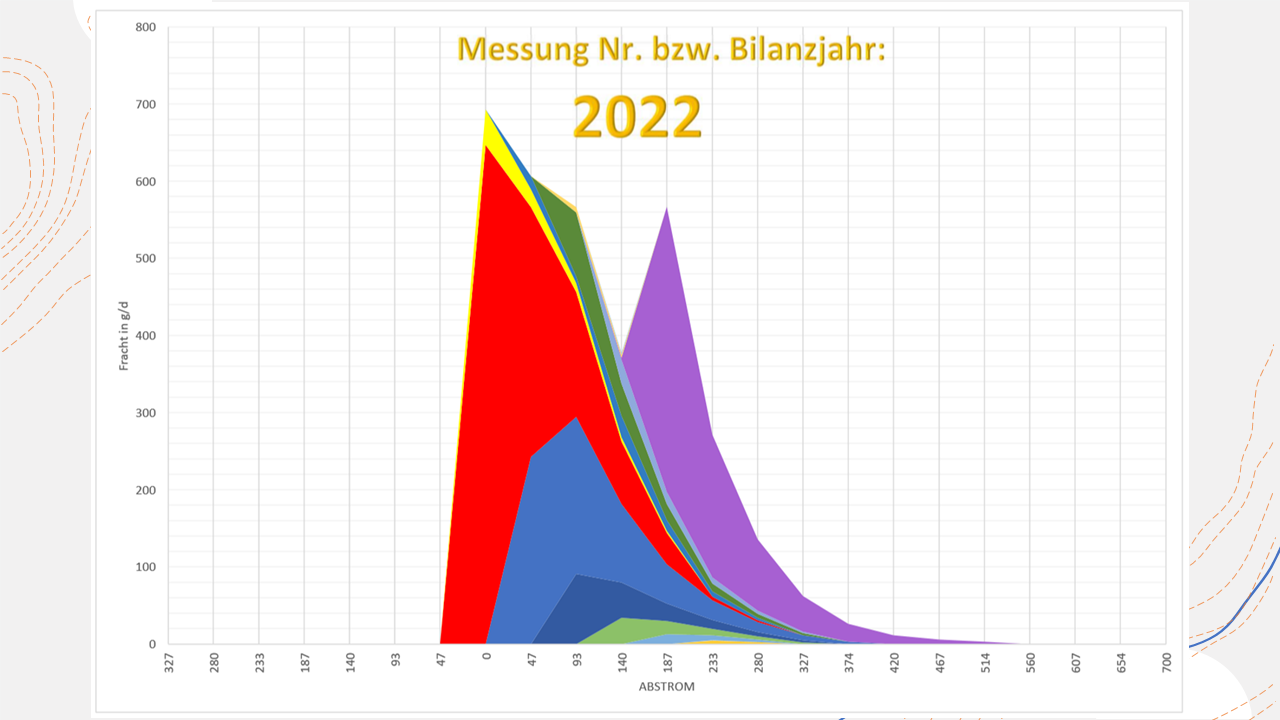
The daily load in a grid cell or a section of streamtube is determined by multiplying the estimated or measured pollutant concentration in the respective cell by the downstream groundwater discharge (QKGW) of the cell. The downstream groundwater discharge indicates how much groundwater flows through the cell, and thus, how much pollutant is transported away.
The summation of daily loads of individual grid cells in the respective balance planes or transects results in the evaluated load. This diagram allows one to read off the amount of load that is flowing out of any given balance plane. For example, after approximately 300 m, a pollutant load of 100 g/d is still flowing out. Transects or balance planes are cross-sections that are drawn perpendicular to the groundwater flow direction.
Concentration profile in the direction of groundwater flow
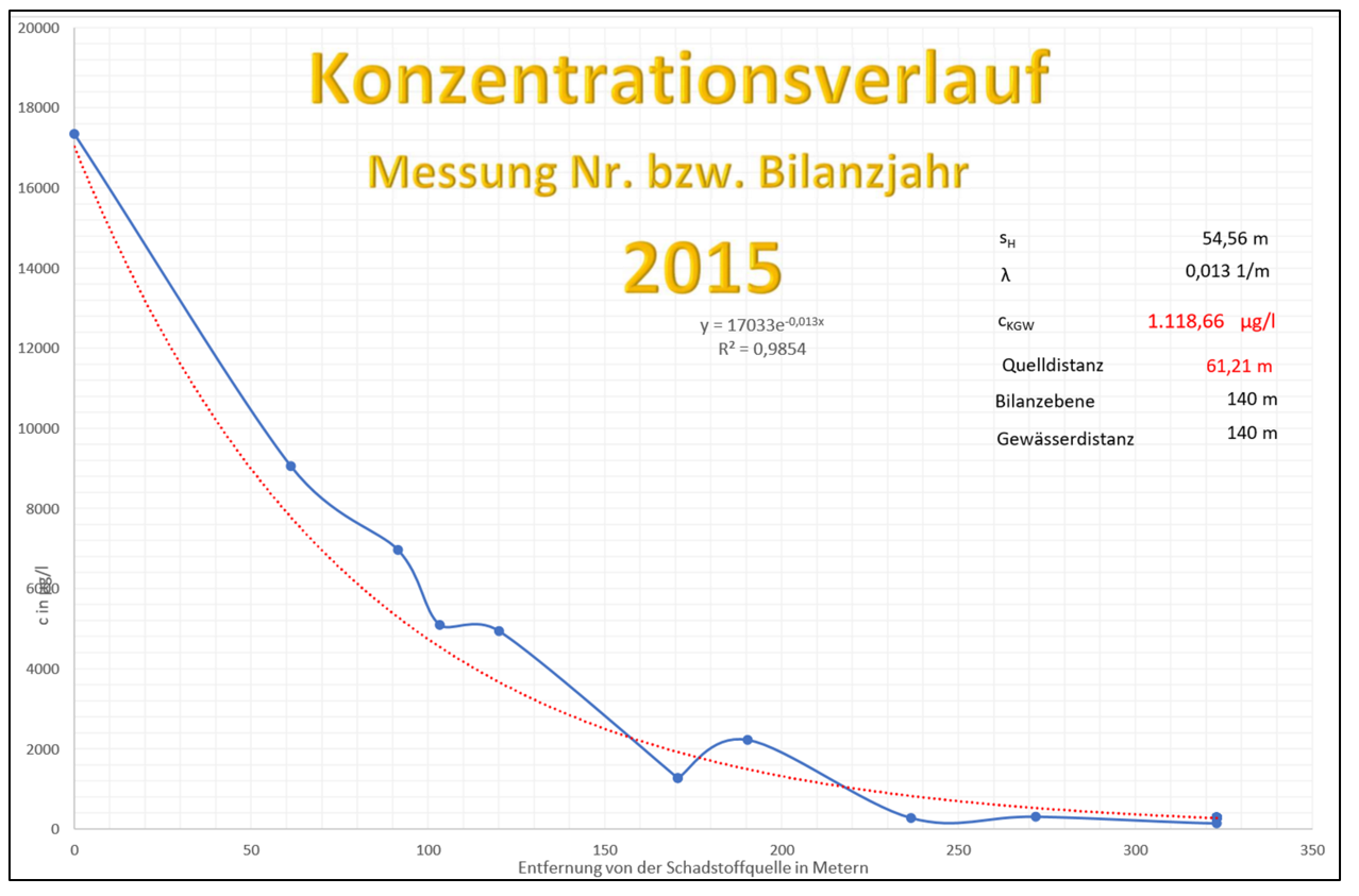
The graphical representation of pollutant degradation along a flow path usually shows, when groundwater monitoring wells are positioned properly along a flow line, that the pollutant degradation can be very well described by the exponential function.
The amplitude deviation from the exponential trendline is a good measure for the presence of homogeneous or anisotropic conditions in an aquifer.
The pollutant degradation coefficient in the exponential function is the quantity that describes how fast a pollutant is degraded in the direction of groundwater flow. The pollutant degradation coefficient is different for various pollutants and various hydrogeological conditions. A high pollutant degradation coefficient means that the pollutant is degraded after a short flow path, while a low pollutant degradation coefficient means that the pollutant degradation takes a longer flow path. The exact rate of pollutant degradation depends on various factors, such as the type of pollutant, the conditions of the degradation process, and the existing microorganisms.
In the pollutant degradation equation, all sorption, desorption, diffusion, and biological degradation processes are integrated into the proportionality factor depending on the physical and chemical properties of the respective pollutant (viscosity, density, water solubility, volatilization, etc.) for the entire model or reaction space, for the sake of simplicity.
Long-term trend for the average pollutant concentration in source and plume
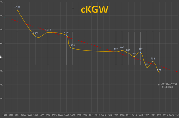
In addition, I offer the possibility to display the development over all observation years for all groundwater monitoring wells and for the average contact groundwater contamination (cCGW) in a diagram, in which the long-term trend can also be assessed. In the example, the linear trend is decreasing. The coefficient of determination of the linear trend is 85%. The long-term decrease in pollutants is clearly visible. I offer the possibility to perform corresponding analyses for each observed groundwater monitoring well.
Long-term trend for a groundwater monitoring well
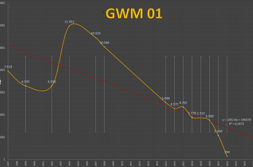
In the example, the linear trend for the GW monitoring well 01 is also decreasing. However, the coefficient of determination of the linear trend is only 57%.
Forecast-diagram with confidence intervals.
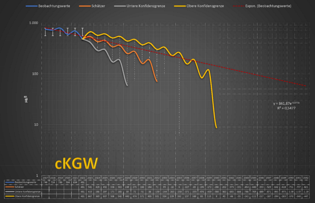
Confidence intervals are a measure of how certain the prediction is. The confidence intervals depend on the sample size and the dispersion of the data. Generally, the larger the sample size and the lower the dispersion of the data, the closer the confidence intervals are together.
With the five years following the reporting year, I calculate the lower confidence limit, the estimator (average confidence limit), and the upper confidence limit, provided that six observations are available for this annual interval.
In our example, the lower confidence limit for the mean groundwater contamination concentration (cKGW) falls below the threshold for negligible impact (GFS) in 2030, the estimator (average confidence limit) in 2034, and the upper confidence limit in 2040. This suggests that by 2040, a "good" groundwater status (cKGW less than GFS) could be achieved at the latest.
Radiation diagram
[B 20] Bestimmung von Redoxzonen in einem mineralölbelasteten Grundwasserleiter, Rudolf Huth, Rainer Hartmann, Michaela Kiesel, Wilhelm Pyka, Annette Stallauer
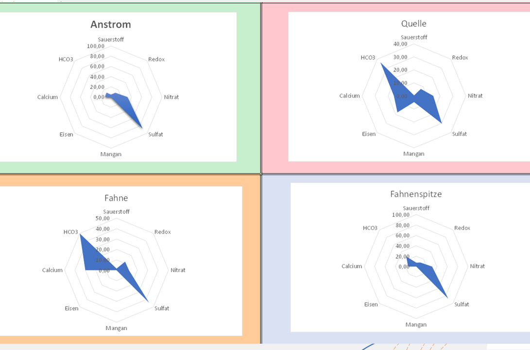
Pollutants can be oxidized by microorganisms and serve as a source of carbon and energy. Due to different environmental conditions in groundwater, different redox zones are formed. Under aerobic conditions, oxygen acts as an electron donor and acceptor. Electron acceptors play an important and essential role in the energy production of cells. Electron acceptors are chemical compounds that are able to accept electrons and become electrically positively charged. In redox reactions, electrons are transferred from a reducing agent to an oxidizing agent. After the dissolved oxygen in the water is consumed, the oxygen atoms are respired by nitrate, iron and manganese oxides, and sulfate. After all electron acceptors are consumed, the methanogenic pollutant degradation takes place, which produces CO2 and methane, leading to an increase in HCO3 in groundwater, which shifts the calcite-carbonic acid equilibrium. This means the formation of soluble Ca(HCO3)2 from insoluble CaCO3 and thus an increase in the levels of Ca2+ in the groundwater. The degradation of hydrocarbons by microorganisms thus leads to a characteristic redox zoning and a change in secondary parameters such as calcium and bicarbonate. An evaluation using a radiation diagram presupposes, of course, that the respective parameters have also been measured in the measuring points representative for source, plume and plume tip.
Representation of calculation results in graphical information systems, such as QGIS
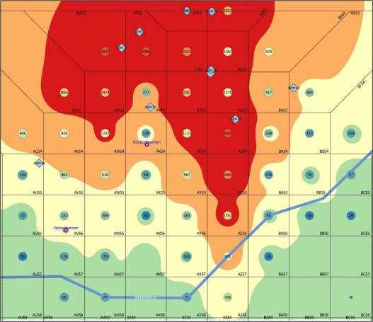
Fiktiver Grundwasserschaden in der Porta Nigra in Trier
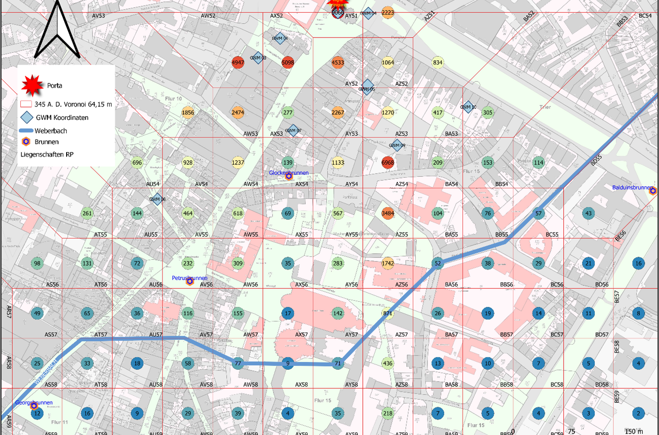
The results of concentration calculations were plotted on the map. To draw the grid, a Voronoi or Thiessen polygon was generated using QGIS based on the imported concentrations. The grid cell dimensions correspond to the calculated half-life distances.
For example, it could now be examined in which areas indoor air measurements in the basements would need to be conducted if it was determined that above a certain concentration threshold, there is a risk that VOCs from groundwater could diffuse into the indoor air of the basements. I can also show particularly sensitive areas, such as kindergartens, sports halls, etc. separately on the map to locate these areas.
Inverse distance weighting (IDW)
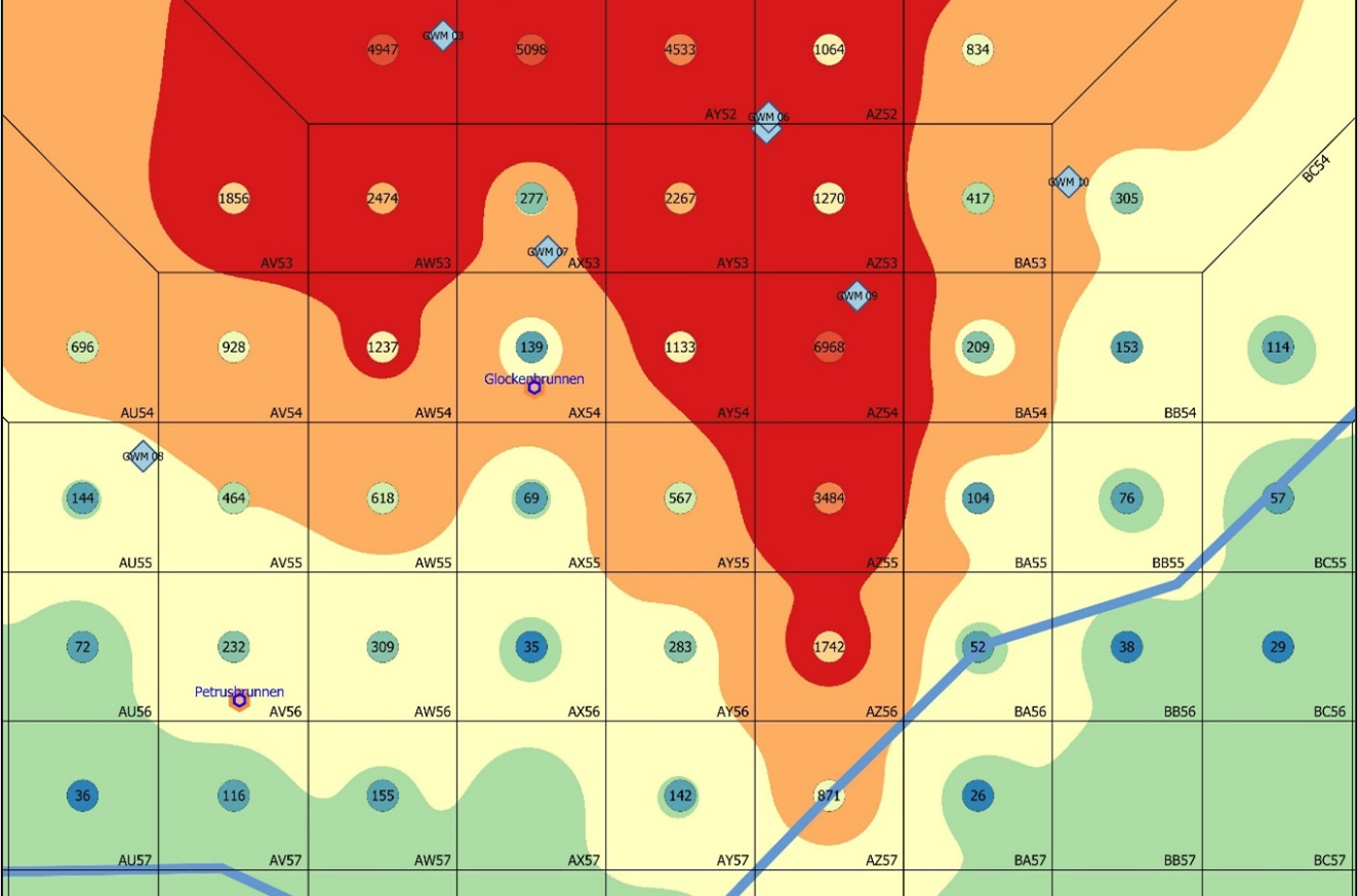
In the above example, an inverse distance weighting (IDW) was applied to the concentrations exported from QGIS, resulting in a smooth color gradient from the raster representation of the contamination plume. The example shows that by using a combination of two methods, a better "picture" can be obtained and a deeper understanding of the processes can be gained through such analyses. It should be noted that the true contour of the contaminant plume can never be determined with absolute certainty, no matter how many groundwater monitoring wells or more accurate modeling programs are used. As the old miner's saying goes, "It's dark in front of the pickaxe."
Closing gaps in the garden fence
[L 02] Gillbricht Christian A., Radmann Kai-Justin, Anmerkungen zur Schätzung von Schadstofffrachten im Grundwasser, Altlasten Spektrum (5/2020)
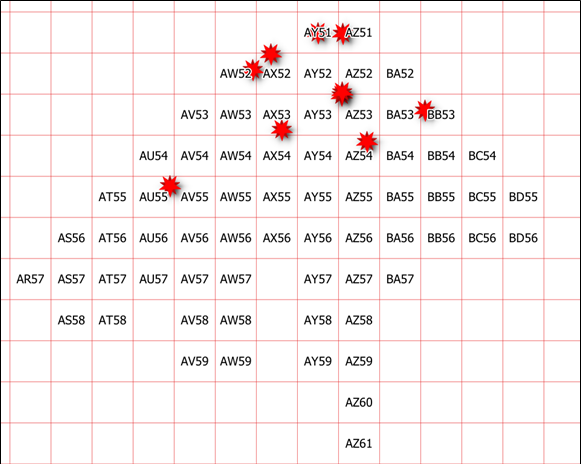
As shown in the above figure, there are no groundwater monitoring wells (red stars) in the conduit or in columns AV and BA. In other words, two boards are missing from the garden fence [L02]. A groundwater monitoring well in column AV would be desirable to monitor the pollutant situation in the area of the Petrusbrunnen on the Hauptmarkt in grid cell AV56, as it in our example draws its water from the polluted aquifer and is used for drinking water purposes, as are the wells in Glockenstraße (AX54), Georgsbrunnen (AS59) and Balduinsbrunnen (BE55) in the fictitious example. However, a danger can be ruled out for the Georgsbrunnen in grid cell AS59, as the Weberbach runs between this receptor and the source of pollution and acts as a dividing line or terminator, preventing pollutant spreading in the southern downstream direction.

My Promise
I will handle your assignment quickly and reliably as your partner for environmental consulting and environmental engineering.
I guarantee you a fast and discreet processing of all your assigned tasks.
Contact: TR-EX Consulting "Water & Waste & Soil"
TTelefon: +49 157 30247862
E-mail: Karlheinz.Mesenich@trex73.de
Dipl. Ing. (FH) Karlheinz Mesenich, Südallee 34c, 54290 Trier